The journey of a Select query through the insides of Postgres
Before the conference PG Day'16 Russia remained a few days, the schedule can be viewed on our website. We are working up a sweat, but nonetheless have time to cook for you translations of the most interesting materials about PostgreSQL. Today we represent to your attention translation of the article Pat Shaughnessy about the behavior of a Select query.
In the summer preparing for this presentation I decided to explore some parts of the source code of PostgreSQL on C. I ran a very simple select query and observed that Postgres doing with it, using an lldb debugger C. As Postgres understand my request? He found the data I was looking for?

This post is an informal journal of my journey through the insides of PostgreSQL. I will describe passed my way and what I saw in the process. I use a series of simple conceptual diagrams to explain how Postgres fulfilled my request. If you understand C, I'll also leave you a few landmarks and signposts you can look, if you suddenly decide to dig in the guts of Postgres.
The source code of PostgreSQL delighted me. It was clean, well-documented and easy to understand. Find out for yourself how Postgres works from the inside, joining me in the journey into the depths of the tool that you use every day.
the
Here is an example query of the the first half of my presentation. We will follow Postgresol while he searches for Captain Nemo's
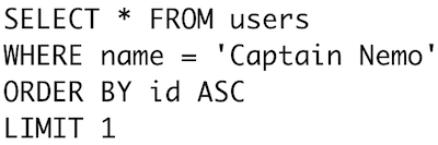
Find one single name in the text column should be simple enough, right? We will hold tight to this select query, exploring the insides of Postgres as deep sea divers hold onto the rope to find the way back to the surface.
the
What makes Postgres with this SQL string? He understands what we mean? As it learns what data are we looking for?
Postgres processes each SQL command, which we sent him in four steps.

First PostgreSQL produces a syntax analysis (“parsing”) our SQL query and converts it into a number of in-memory data structures the C language — the parse tree (parse tree). Further, Postgres analyzes and overwrite our request, optimizing and simplifying it using a series of complex algorithms. After that, it generates plan to search our data. Like people with obsessive-compulsive disorder, who go out of the house, while his portfolio will be carefully Packed, Postgres will not start our inquiry, yet it doesn't have a plan. Finally, Postgres does our request. In this presentation I will briefly touch on the first three steps, and then focus on the last one: execution.
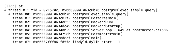
The C function inside Postgres that performs this four-step process, called exec_simple_query. You can find a link to it below along with an lldb trace, which shows the details of exactly when and how Postgres calls exec_simple_query.

the

the
As Postgres understands SQL string that we sent him? As he finds the meaning of key words and expressions in our SQL select query? Through a process called parse (parsing). Postgres convert our SQL string into an internal data structure that it understands the parse tree.
It turns out that Postgres uses the same parsing technology that Ruby, namely — a parser generator called Bison. Bison running during the build process of Postgres and generates the code of a parser based on some grammar rules. The generated code of the parser is that it works inside of Postgres when we send him a SQL command. Every grammatical rule is called when the generated parser finds a matching pattern or syntax in the SQL string and inserts a new memory structure in C tree parsing.
Today I'm not going to waste time on a detailed explanation of how the algorithm of parsing. If you are interested in these topics, I advise you to read my book, Ruby Under a Microscope. In the first Chapter I consider in detail an example of the parsing algorithm is O used Bison and Ruby. Postgres parses the SQL query in exactly the same way.
Using an lldb and activating some logimouse C code, I watched as the parser of Postgres created the following parse tree for our query to find Captain Nemo's

On top is a node representing a complete SQL query, and below that are child nodes, or branches that represent the different pieces of the SQL syntax query: target list (column list) from (list of tables) the where clause, sort order and number of entries.
If you want to know more about how Postgres parses SQL queries, follow procedures from exec_simple_query through another C function called pg_parse_query.
the
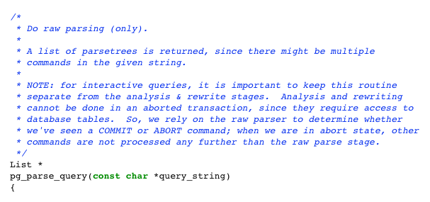

As you can see in the source code of Postgres a lot of useful and detailed reviews that not only explain what is happening, but also point out important design decisions.
the
The parse tree above probably looks familiar — it's almost exactly the same abstract syntax tree (AST), which in ActiveRecord we have seen before. Remember the first part of the presentation: ActiveRecord generated by our select query about Captain Nemo, when we executed this query in Ruby:
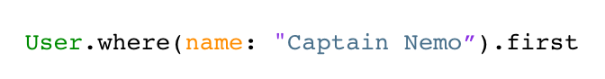
We saw that ActiveRecord has created an internal representation of the AST when we called methods such as where and first. Later (see the second post) we watched as the gem Arel AST is converted to our example of a select query using the algorithm based on the visitor pattern.
If you think about it, very ironic that the first thing Postgres does with your SQL query — convert it from string back to AST. The process of parsing Postgres undo all that ActiveRecord was doing, all the hard work done by the Arel gem, in vain! The only reason to create a SQL string was to Postgres on the network. But as soon as Postgres received the request, he converted it back into an AST which is much more convenient and useful way of representing queries.
Knowing this, you may ask: isn't there a better way? Is there no other way to explain the conceptual Postgres what data we need without writing SQL query? Without learning complex SQL or additional overheads due to the use of ActiveRecord and Arel? It seems a monstrous waste of time to go such a long way, creating a SQL string from an AST only in order again to convert it back to AST. Maybe we should instead use a NoSQL solution?
Of course, the AST used by Postgres, very different from the AST used by ActiveRecord. In ActiveRecord AST consists of objects Ruby and Postgres — from the in-memory structures of the language C. the Idea of one, but the implementation is very different.
the
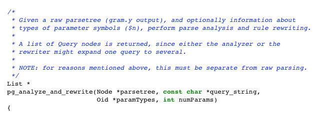
As soon as Postgres generated the parse tree, it converts it into another tree, using another set of nodes. It is known as the query tree. Returning to the C function, exec_simple_query, you can see that then another function is called C — pg_analyze_and_rewrite.
the

If you do not go into the details, the process of analyzing and rewriting applies a series of complex algorithms and heuristics to try to optimize and simplify your SQL query. If you have completed a complex select query with nested queries and multiple inner and outer join, the scope for optimization is huge. It is possible that Postgres will reduce the number of subqueries or associations to produce a simpler query that will be faster.
For our simple select query pg_analyze_and_rewrite created here is the query tree:
I will not pretend to understand the details of the algorithms behind pg_analyze_and_rewrite. I just noticed that for our example, the query tree is very similar to the parse tree. This means that the select query was so simple that Postgres was not able to make it even easier.
the
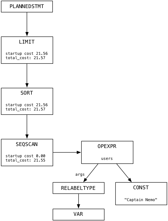
The last thing Posgres makes before starting to execute the query, creates a plan. This process involves creating a third tree node which represent a list of instructions for Postgres. Here is a tree plan for our select query:
Imagine that each node in the tree plan — it is some machine or worker. The tree plan is based on the pipeline data or the conveyor belt in a factory. In my simple example, the tree has only one branch. Each node in the plan tree takes the data from the output of the underlying host, processes them, and returns the result as initial data for the node above. In the next paragraph we follow Postgresol while it will carry out the plan.
The C function that starts the planning process of a query is called pg_plan_queries.
the


Note the startup_cost and total_cost values at each node. Postgres uses these values to estimate how long it will take to execute the plan. You don't need to use the C debugger to see the execution plan of your query. Just add at the beginning of the query the SQL command EXPLAIN. Here it is:

This is a great way to understand that Postgres internally doing with one of your requests and why it might be slow or inefficient, despite the complex scheduling algorithms in pg_plan_queries.
the
At this point, Postgres subjected to your SQL string to parse and convert it back to AST. Then he optimized and rewritten, probably, simplifying. After that, Postgres have written a plan that will follow to find and return the data that you are looking for. Finally, it's time for Postgres to assist you with your request! How would he do it? Following the plan, of course!
Let's start from the top of the plan tree and move down. If you omit the root node, the first worker, which Postgres uses for our request of Captain Nemo, is called Limit. The node Limit, as you might guess, executes the SQL command LIMIT, which restricts the result to a specific number of records. Also, this plan node executes the command OFFSET, which initiates a window result set, starting with the specified string.

When you first call node Limit Postgres calculates what should be the values for limit and offset, as they can be bound to the result of some dynamic calculation. In our example, offset is 0 and limit — 1.
Further, the Limit plan node repeatedly calls subplan — in our case it is Sort — until it reaches the value of offset

In our example the offset is zero, so this loop will load the first data value and stop iteration. Then Postgres returns the last data value is loaded from subplana causing or parent plan. For us this will be the first value of subplana.
Finally, when Postgres will continue to cause the node Limit, it will transfer the data values of subplana one:
Since in our example, the limit is equal to 1, Limit will immediately return NULL, showing a higher plan, that there is no more data available.
Postgres performs the node Limit using the code from the file called nodeLimit.with
the
You can see that the source code of Postgres uses such words as tuple (set of values, one from each column) and subplan. In this example, subplan is a Sort node, which is located in the plan under Limit.
the
Where are data values that filters out Limit? From a node of Sort located under the Limit in the tree plan. Sort loads the data values from their subplan and returns them to the calling node Limit. Here's what Sort does when the node Limit causes it in the first time to obtain first value data:

As you can see, the Sort functions not as the Limit. It immediately loads all of the available data from subplan into the buffer before any return. Then it sorts the buffer using the algorithm Quicksort and, finally, returns the first sorted value.
For the second and subsequent calls, Sort simply returns additional values from the sorted buffer, and did not need again to call subplan:

The Sort plan node executes a C function called ExecSort:
the

the
Where ExecSort takes the values? Your sublane — SeqScan node, located at the bottom of the plan tree. SeqScan stands for sequential scan (sequential scan), which implies a view of all the values in a table and return values that match the specified filter. To understand how scanning works with our filter, let's imagine the user table filled with fictitious names, and will try to find Captain Nemo.

Postgres begins with the first entry in the table (which in the source code of Postgres called relation) and starts the Boolean expression from the plan tree. Simply put, Postgres asks the question: "is This Captain Nemo?" As Laurianne Goodwin — it's not Captain Nemo, Postgres moves to the next record.

No, Candace is also not Captain Nemo. Postgres continues:
... and in the end finds Captain Nemo!
Postgres performs a SeqScan node using a C function called ExecSeqScan.
the

the
Here we come to the end! We followed a simple select query all the way through the insides of Postgres and saw how he was subjected to a syntax analysis, has been rewritten, planned and finally executed. After executing many thousands of lines of code in C Postgres found the data we were looking for! Now all he has left to do is return a row of Captain Nemo back into our Rails application and ActiveRecord can create a Ruby object. Finally, we can return to the surface of our application.
But Postgres won't stop! Instead just return the data, he continues to scan the user table, although we have found Captain Nemo:

What happens? Why Postgres spends his time continuing to search, despite the fact that you already found the necessary data?
The answer lies in the tree plan node, Sort. Remember that to sort all users ExecSort first loads all the values in the buffer, repeatedly triggering subplan, while the values over. This means that ExecSeqScan will continue to scan until the end of the table, until all the appropriate user. If our table contain thousands or even millions of records (imagine that we are working in Facebook or Twitter), ExecSeqScan would have to repeat the loop for all user accounts and to perform a comparison for each of them. Obviously this is slow and inefficient, and we will increasingly slow down as the table will add new user accounts.
If we only have one record of Captain Nemo, ExecSort "sort" and this is the only appropriate entry, and ExecLimit run it through your filter offset/limit... but only after ExecSeqScan will be held for all names.
the
How to solve this problem? What to do if to run our SQL queries on the users table requires more and more time? The answer is simple: we create the index.
In the next and last post in this series we will learn how to create Postgres indexes and avoid using ExecSeqScan. But most importantly I will show you how looks the index in Postgres: how it works and why it speeds up like this.
Article based on information from habrahabr.ru
In the summer preparing for this presentation I decided to explore some parts of the source code of PostgreSQL on C. I ran a very simple select query and observed that Postgres doing with it, using an lldb debugger C. As Postgres understand my request? He found the data I was looking for?
This post is an informal journal of my journey through the insides of PostgreSQL. I will describe passed my way and what I saw in the process. I use a series of simple conceptual diagrams to explain how Postgres fulfilled my request. If you understand C, I'll also leave you a few landmarks and signposts you can look, if you suddenly decide to dig in the guts of Postgres.
The source code of PostgreSQL delighted me. It was clean, well-documented and easy to understand. Find out for yourself how Postgres works from the inside, joining me in the journey into the depths of the tool that you use every day.
the
In search of Captain Nemo
Here is an example query of the the first half of my presentation. We will follow Postgresol while he searches for Captain Nemo's
Find one single name in the text column should be simple enough, right? We will hold tight to this select query, exploring the insides of Postgres as deep sea divers hold onto the rope to find the way back to the surface.
the
the Picture
What makes Postgres with this SQL string? He understands what we mean? As it learns what data are we looking for?
Postgres processes each SQL command, which we sent him in four steps.
First PostgreSQL produces a syntax analysis (“parsing”) our SQL query and converts it into a number of in-memory data structures the C language — the parse tree (parse tree). Further, Postgres analyzes and overwrite our request, optimizing and simplifying it using a series of complex algorithms. After that, it generates plan to search our data. Like people with obsessive-compulsive disorder, who go out of the house, while his portfolio will be carefully Packed, Postgres will not start our inquiry, yet it doesn't have a plan. Finally, Postgres does our request. In this presentation I will briefly touch on the first three steps, and then focus on the last one: execution.
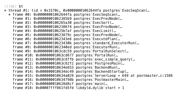
The C function inside Postgres that performs this four-step process, called exec_simple_query. You can find a link to it below along with an lldb trace, which shows the details of exactly when and how Postgres calls exec_simple_query.
the
exec_simple_query
view on postgresql.orgthe
parse
As Postgres understands SQL string that we sent him? As he finds the meaning of key words and expressions in our SQL select query? Through a process called parse (parsing). Postgres convert our SQL string into an internal data structure that it understands the parse tree.
It turns out that Postgres uses the same parsing technology that Ruby, namely — a parser generator called Bison. Bison running during the build process of Postgres and generates the code of a parser based on some grammar rules. The generated code of the parser is that it works inside of Postgres when we send him a SQL command. Every grammatical rule is called when the generated parser finds a matching pattern or syntax in the SQL string and inserts a new memory structure in C tree parsing.
Today I'm not going to waste time on a detailed explanation of how the algorithm of parsing. If you are interested in these topics, I advise you to read my book, Ruby Under a Microscope. In the first Chapter I consider in detail an example of the parsing algorithm is O used Bison and Ruby. Postgres parses the SQL query in exactly the same way.
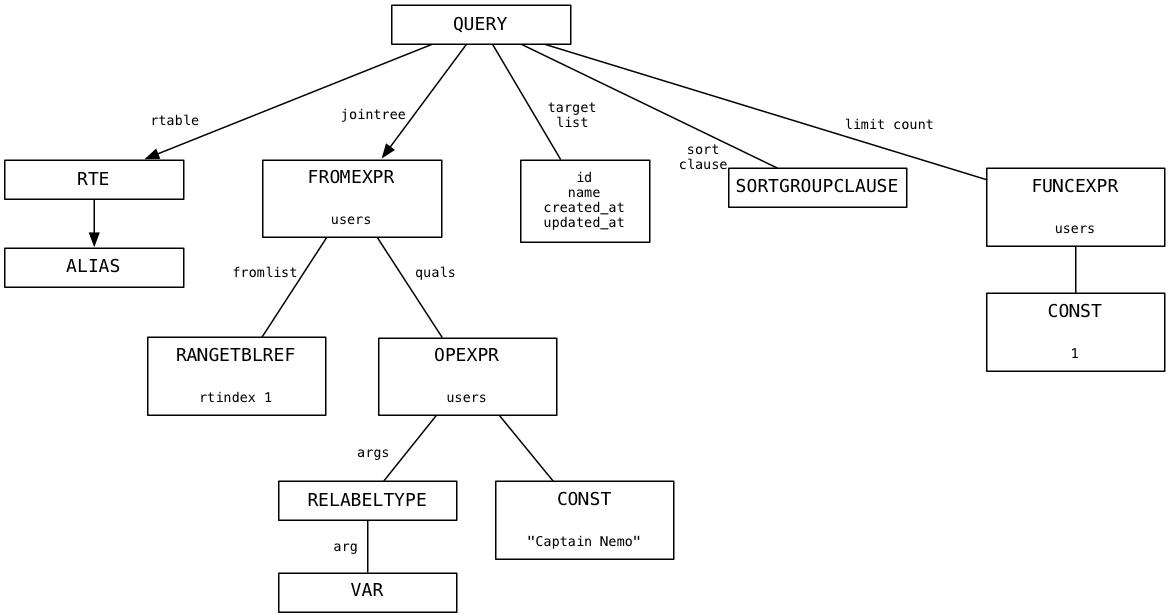
Using an lldb and activating some logimouse C code, I watched as the parser of Postgres created the following parse tree for our query to find Captain Nemo's
On top is a node representing a complete SQL query, and below that are child nodes, or branches that represent the different pieces of the SQL syntax query: target list (column list) from (list of tables) the where clause, sort order and number of entries.
If you want to know more about how Postgres parses SQL queries, follow procedures from exec_simple_query through another C function called pg_parse_query.
the
pg_parse_query
view on postgresql.orgAs you can see in the source code of Postgres a lot of useful and detailed reviews that not only explain what is happening, but also point out important design decisions.
the
All that work down the drain
The parse tree above probably looks familiar — it's almost exactly the same abstract syntax tree (AST), which in ActiveRecord we have seen before. Remember the first part of the presentation: ActiveRecord generated by our select query about Captain Nemo, when we executed this query in Ruby:
We saw that ActiveRecord has created an internal representation of the AST when we called methods such as where and first. Later (see the second post) we watched as the gem Arel AST is converted to our example of a select query using the algorithm based on the visitor pattern.
If you think about it, very ironic that the first thing Postgres does with your SQL query — convert it from string back to AST. The process of parsing Postgres undo all that ActiveRecord was doing, all the hard work done by the Arel gem, in vain! The only reason to create a SQL string was to Postgres on the network. But as soon as Postgres received the request, he converted it back into an AST which is much more convenient and useful way of representing queries.
Knowing this, you may ask: isn't there a better way? Is there no other way to explain the conceptual Postgres what data we need without writing SQL query? Without learning complex SQL or additional overheads due to the use of ActiveRecord and Arel? It seems a monstrous waste of time to go such a long way, creating a SQL string from an AST only in order again to convert it back to AST. Maybe we should instead use a NoSQL solution?
Of course, the AST used by Postgres, very different from the AST used by ActiveRecord. In ActiveRecord AST consists of objects Ruby and Postgres — from the in-memory structures of the language C. the Idea of one, but the implementation is very different.
the
Analysis and rewriting
As soon as Postgres generated the parse tree, it converts it into another tree, using another set of nodes. It is known as the query tree. Returning to the C function, exec_simple_query, you can see that then another function is called C — pg_analyze_and_rewrite.
the
pg_analyze_and_rewrite
view on postgresql.orgIf you do not go into the details, the process of analyzing and rewriting applies a series of complex algorithms and heuristics to try to optimize and simplify your SQL query. If you have completed a complex select query with nested queries and multiple inner and outer join, the scope for optimization is huge. It is possible that Postgres will reduce the number of subqueries or associations to produce a simpler query that will be faster.
For our simple select query pg_analyze_and_rewrite created here is the query tree:
I will not pretend to understand the details of the algorithms behind pg_analyze_and_rewrite. I just noticed that for our example, the query tree is very similar to the parse tree. This means that the select query was so simple that Postgres was not able to make it even easier.
the
Plan
The last thing Posgres makes before starting to execute the query, creates a plan. This process involves creating a third tree node which represent a list of instructions for Postgres. Here is a tree plan for our select query:
Imagine that each node in the tree plan — it is some machine or worker. The tree plan is based on the pipeline data or the conveyor belt in a factory. In my simple example, the tree has only one branch. Each node in the plan tree takes the data from the output of the underlying host, processes them, and returns the result as initial data for the node above. In the next paragraph we follow Postgresol while it will carry out the plan.
The C function that starts the planning process of a query is called pg_plan_queries.
the
pg_plan_queries
view on postgresql.orgNote the startup_cost and total_cost values at each node. Postgres uses these values to estimate how long it will take to execute the plan. You don't need to use the C debugger to see the execution plan of your query. Just add at the beginning of the query the SQL command EXPLAIN. Here it is:
This is a great way to understand that Postgres internally doing with one of your requests and why it might be slow or inefficient, despite the complex scheduling algorithms in pg_plan_queries.
the
Execution plan node Limit
At this point, Postgres subjected to your SQL string to parse and convert it back to AST. Then he optimized and rewritten, probably, simplifying. After that, Postgres have written a plan that will follow to find and return the data that you are looking for. Finally, it's time for Postgres to assist you with your request! How would he do it? Following the plan, of course!
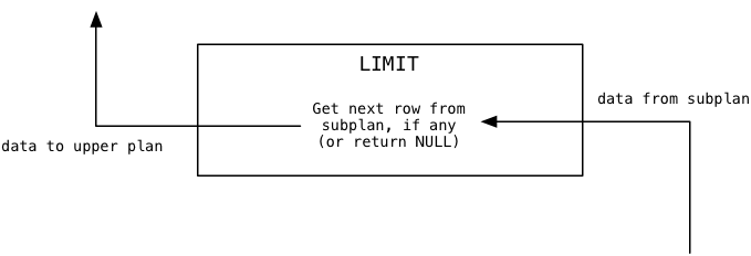
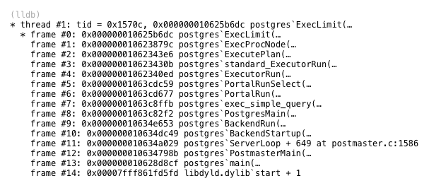
Let's start from the top of the plan tree and move down. If you omit the root node, the first worker, which Postgres uses for our request of Captain Nemo, is called Limit. The node Limit, as you might guess, executes the SQL command LIMIT, which restricts the result to a specific number of records. Also, this plan node executes the command OFFSET, which initiates a window result set, starting with the specified string.
When you first call node Limit Postgres calculates what should be the values for limit and offset, as they can be bound to the result of some dynamic calculation. In our example, offset is 0 and limit — 1.
Further, the Limit plan node repeatedly calls subplan — in our case it is Sort — until it reaches the value of offset
In our example the offset is zero, so this loop will load the first data value and stop iteration. Then Postgres returns the last data value is loaded from subplana causing or parent plan. For us this will be the first value of subplana.
Finally, when Postgres will continue to cause the node Limit, it will transfer the data values of subplana one:
Since in our example, the limit is equal to 1, Limit will immediately return NULL, showing a higher plan, that there is no more data available.
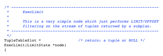
Postgres performs the node Limit using the code from the file called nodeLimit.with
the
ExecLimit
view on postgresql.orgYou can see that the source code of Postgres uses such words as tuple (set of values, one from each column) and subplan. In this example, subplan is a Sort node, which is located in the plan under Limit.
the
Execution plan node Sort
Where are data values that filters out Limit? From a node of Sort located under the Limit in the tree plan. Sort loads the data values from their subplan and returns them to the calling node Limit. Here's what Sort does when the node Limit causes it in the first time to obtain first value data:
As you can see, the Sort functions not as the Limit. It immediately loads all of the available data from subplan into the buffer before any return. Then it sorts the buffer using the algorithm Quicksort and, finally, returns the first sorted value.
For the second and subsequent calls, Sort simply returns additional values from the sorted buffer, and did not need again to call subplan:
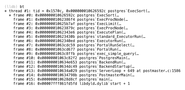
The Sort plan node executes a C function called ExecSort:
the
ExecSort
view on postgresql.orgthe
Execution plan node SeqScan
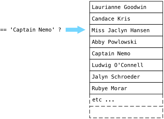
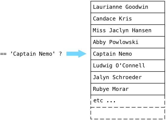
Where ExecSort takes the values? Your sublane — SeqScan node, located at the bottom of the plan tree. SeqScan stands for sequential scan (sequential scan), which implies a view of all the values in a table and return values that match the specified filter. To understand how scanning works with our filter, let's imagine the user table filled with fictitious names, and will try to find Captain Nemo.
Postgres begins with the first entry in the table (which in the source code of Postgres called relation) and starts the Boolean expression from the plan tree. Simply put, Postgres asks the question: "is This Captain Nemo?" As Laurianne Goodwin — it's not Captain Nemo, Postgres moves to the next record.
No, Candace is also not Captain Nemo. Postgres continues:
... and in the end finds Captain Nemo!
Postgres performs a SeqScan node using a C function called ExecSeqScan.
the
ExecSeqScan
view on postgresql.orgthe
What are we doing wrong?
Here we come to the end! We followed a simple select query all the way through the insides of Postgres and saw how he was subjected to a syntax analysis, has been rewritten, planned and finally executed. After executing many thousands of lines of code in C Postgres found the data we were looking for! Now all he has left to do is return a row of Captain Nemo back into our Rails application and ActiveRecord can create a Ruby object. Finally, we can return to the surface of our application.
But Postgres won't stop! Instead just return the data, he continues to scan the user table, although we have found Captain Nemo:
What happens? Why Postgres spends his time continuing to search, despite the fact that you already found the necessary data?
The answer lies in the tree plan node, Sort. Remember that to sort all users ExecSort first loads all the values in the buffer, repeatedly triggering subplan, while the values over. This means that ExecSeqScan will continue to scan until the end of the table, until all the appropriate user. If our table contain thousands or even millions of records (imagine that we are working in Facebook or Twitter), ExecSeqScan would have to repeat the loop for all user accounts and to perform a comparison for each of them. Obviously this is slow and inefficient, and we will increasingly slow down as the table will add new user accounts.
If we only have one record of Captain Nemo, ExecSort "sort" and this is the only appropriate entry, and ExecLimit run it through your filter offset/limit... but only after ExecSeqScan will be held for all names.
the
next time
How to solve this problem? What to do if to run our SQL queries on the users table requires more and more time? The answer is simple: we create the index.
In the next and last post in this series we will learn how to create Postgres indexes and avoid using ExecSeqScan. But most importantly I will show you how looks the index in Postgres: how it works and why it speeds up like this.


Comments
Post a Comment